Fort Features: Transit Infrastructure Connectivity
How We Evaluate Potential Industrial Investments Using A Transit Infrastructure Connectivity Score
There is a close connection between industrial real estate and freight transportation due to the nature of the industry’s operations. To understand how attractive a particular area or asset is for investment, we need to model how it fits into the overall freight transportation system. Our transit infrastructure connectivity score is Fort Capital’s way of measuring how well an area is connected to the wider transportation network, including roadways, roadway access points, seaports, marine highways, airports, and railroads. High connectivity is ideal because it means the asset is well-connected and can serve a large area via the most efficient paths of transportation. Inversely, low connectivity means the asset is not as well-connected and may struggle to serve a large area.
Our connectivity metric is important when analyzing potential investments because it helps identify areas that are well-positioned for success. While there has been research on connectivity in small regional transportation systems, there has been less research on large, multi-modal freight transportation networks in industrial real estate. This is because it is difficult to account for different modes of transportation and the costs involved in moving freight across them. However, our methodology includes several methods for evaluating these networks and overcoming these challenges. This connectivity metric is just one of many data points we use in our proprietary deal ranking framework, which helps our team to pinpoint and pursue assets with the best investment opportunity.
While not an easy process to explain, we are sharing our simplified methodology for how we have constructed and use this connectivity metric.
PROCESS 1: DATA EXTRACTION & NORMALIZATION
Overall, the goal of this phase of the process was to identify and normalize data on the routes and access points that are important for freight transportation, including roads, rail lines, airports, seaports, and shipping lanes.
Roadways & Access Points / Rail Lines / Intermodal Terminals / Airports / Seaports
The first step in building a fully comprehensive view of the freight transportation system is identifying the routes and access points to consider. Freight can only travel on specific routes, so it’s important to only consider those routes. The Department of Transportation provides data on the roadways, rail lines, and inland waterways that are designated as freight transportation corridors, as well as the access points to these routes like highway ramps, intermodal terminals, airports, and seaports.
Aerial Routes
Identifying aerial routes is more difficult because they do not have physical infrastructure. However, flight data is heavily tracked and can be used to identify routes between airports. To accurately represent the freight system, only flights between DOT-designated freight airports were considered.
Maritime Shipping Lanes
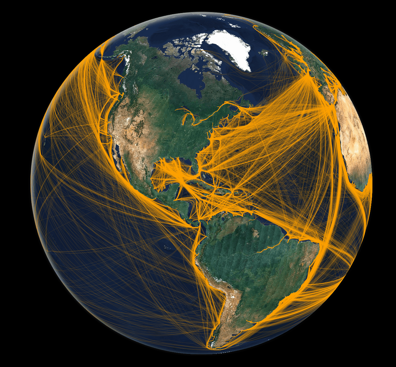
Maritime shipping lanes are also challenging to model because they also do not have physical infrastructure and the routes are not straight lines. To identify unique routes, a dataset of GPS tracking for approximately one million trips was obtained and normalized. The shortest path between each unique port-port relationship was kept to simplify the dataset. To ensure only freight-designated ports were considered, a clustering algorithm was used to identify “trade zones” of ports that were close together and shared connections. The image below is a visual representation of these maritime shipping lanes.
PROCESS 2: CONSTRUCTING A GRAPH NETWORK
The transportation system is like a big puzzle that needs to be pieced together. It’s difficult to ensure all the pieces of the transportation puzzle fit together perfectly. Some parts of the system, like seaports and airports, don’t need to be connected to each other. But other parts, like roads and railroads, do need to be connected. This requires a manual process because the connections have to be very precise.
Graph theory is a way to help us understand how all of the pieces in the fully connected puzzle relate to one another. Basically, it’s a way to represent the relationships between objects. In the transportation system, the points where things move in or out, like airports or seaports, are called “nodes” and the routes that connect them are called “edges.”
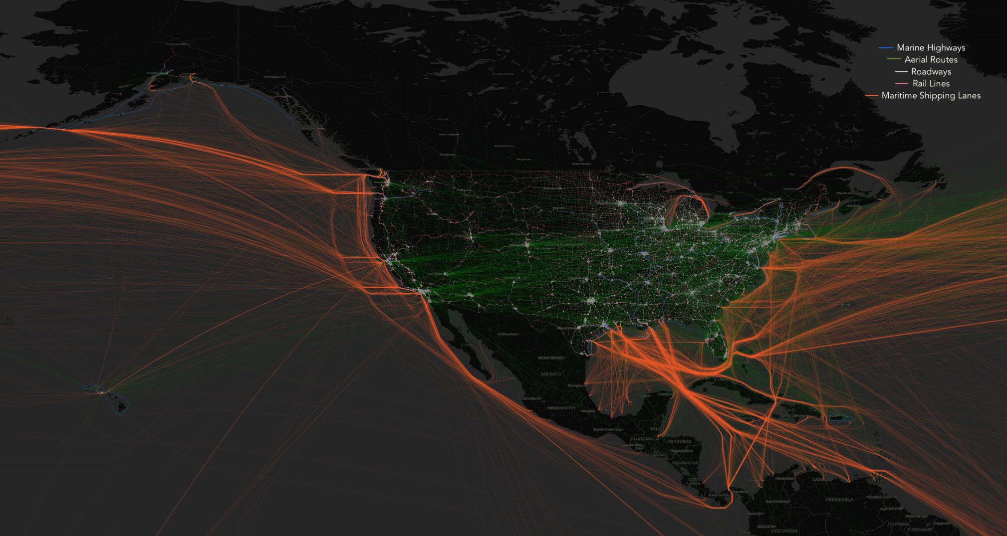
Once everything is connected, we are able to look at the transportation system as a whole and analyze it. The below visual represents the entirety of the United States freight transportation network as it connects domestically and beyond.
PROCESS 3: CONNECTIVITY METRICS & WEIGHTS
To measure how well a transportation network is connected, we use different methods, such as betweenness centrality, closeness centrality, straightness centrality, and node degree. A final, and separate, connectivity analysis is performed on individual buildings that are individualized for the specific location and are not factored into the total network connectivity.
Since analyzing large graphs can be very time-consuming, we use DOT guidance to focus specific modalities within a certain distance from a market’s centroid.
Weights
Prior to initializing an analysis of the selected metrics, we examine the efficiency of a route. Variables that determine the user’s cost to travel a corridor could be traffic congestion, speed limits, weight limits, tolls, price of various commodities, travel time, etc. These variables are difficult to procure and model due to the variable dimensionality and sparseness of reliable data. To overcome this, we took a different approach by analyzing the metric that should be inclusive of the more indirect variables – freight flow.
We assign weights to the edges of the network based on the amount of freight flow on that specific route. The higher the freight flow, the lower the weight. This increases the effectiveness of our analysis because edges with higher freight flow are preferred over those with lower flow.
Betweenness Centrality
Betweenness centrality is a measure that looks at the shortest paths in the network. It calculates how often a node or edge is on the shortest path between any two nodes in the network. This helps us determine the most efficient paths to travel in the network.

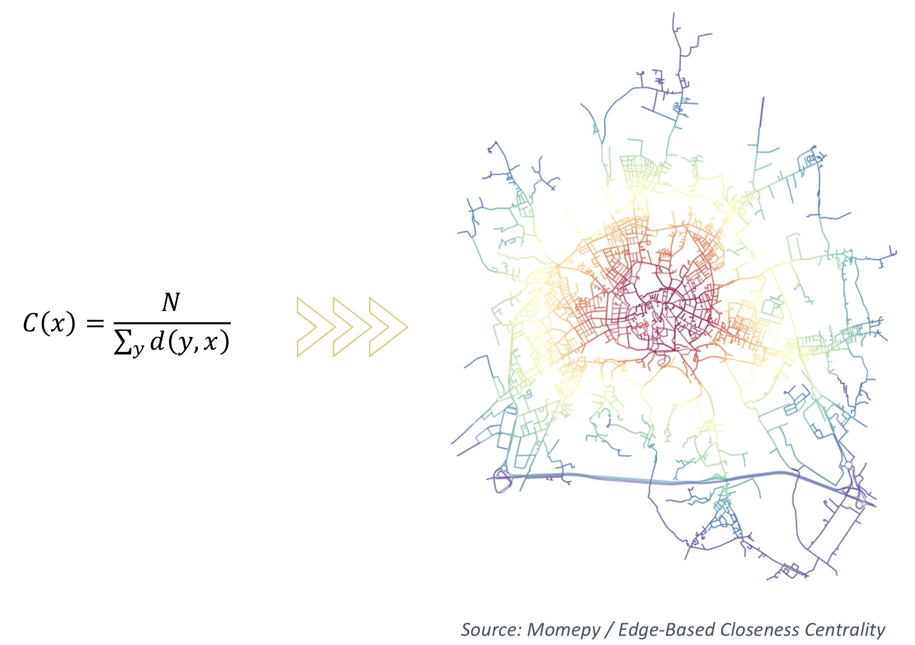
Closeness Centrality
Closeness centrality measures how close a node is to all other nodes in a network. Nodes that are closer to other nodes are more central in the overall network. Clustering is another metric that can show how densely connected access points are in a certain area. This is important in areas with a lot of traffic because it provides multiple options to access the system if the primary route is not available.
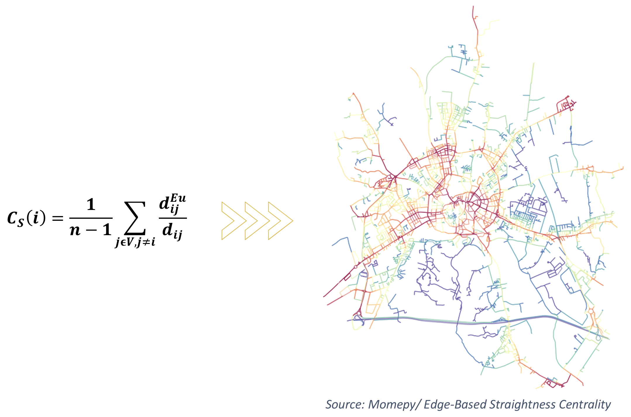
Straightness Centrality
Simply put, straightness centrality is a way of measuring how straight a route is between different points in a transportation network. It looks at the actual distance between nodes as well as the straight-line distance and gives a ratio of the two. A higher value means that the route is more direct. This metric helps to show how easy it is to get from one point to another in the network. It can also be used to measure how complex a route is, with straighter lines indicating a simpler path.
Node Degree
When we rank the importance of different parts of the freight transportation system, we need to make sure we give extra weight to airports and seaports. To do this, we separate these modalities from the main transportation system and consider the number of connections that are present per node. This is called the node degree. It helps us get a more accurate idea of how important these nodes are and also makes it easier to calculate their importance without making the calculation too complicated.
OUTPUT: ASSET CONNECTIVITY SCORE
We can measure how connected an asset is to the overall freight transportation system by calculating how long it takes to drive a truck from the asset to the nearest node in the network. We also consider the asset’s proximity to intermodal terminals, seaports, and airports. This helps us understand how well-connected the asset is locally, nationally, and internationally. Another way we can use this information is to predict how well an asset is connected to places with strong economies. By investing in assets that are well-connected to growing regions, we can capture future demand.
The power of our transit connectivity score is that we are able to apply this to all assets in the entire United States that match our investment criteria, which helps to narrow our list of ideal investments for vetting by our team. We are able to efficiently analyze these top opportunities so that our focus is kept on the potential acquisitions with the most potential upside.
Be sure to subscribe to our newsletter to receive more exclusive content similar to this post from our Economic Strategist.